Programming Computer Vision : Basics
Reading Images
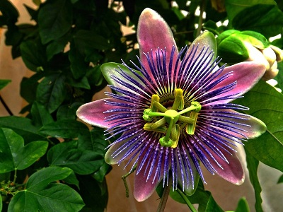
Images can be read using Image class of Python library PIL (Python Imaging Library).
from PIL import Image
im = Image.open('images/flower.jpg')
The return value 'im' is a PIL image object. Thus the following image would be read.
Color conversions
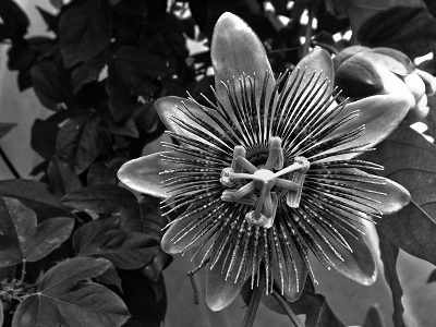
We can use the convert() method for Color conversions. An image can be converted to grayscale using the .convert('L') function where 'L' simply is a mode that defines images as 8-bit pixels of black & white. To learn about other modes, you can visit http://pillow.readthedocs.org/en/3.1.x/handbook/concepts.html.
The library supports transformations between each supported mode and the 'L' and 'RGB' modes. To convert between other modes, you may have to use an intermediate image (typically an “RGB” image).
gray = im.convert('L')
gray.show()
Enhancement
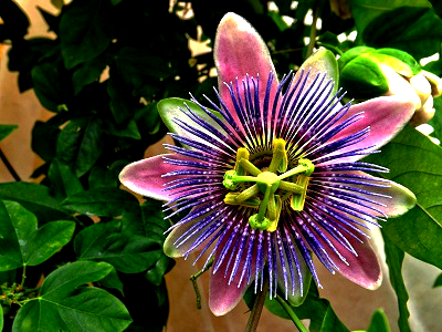
The ImageEnhance module can be used for image enhancement. Once created from an image, an enhancement object can be used to quickly try out different settings. You can adjust contrast, brightness, color balance and sharpness in this way.
from PIL import ImageEnhance

enh = ImageEnhance.Contrast(im)
enh.enhance(1.4).show("30% more contrast")
Converting into other file format
from __future__ import print_function
import os, sys
from PIL import Image

def convertToJPEG():
    for infile in sys.argv[1:]:
        f, e = os.path.splitext(infile)
        outfile = f + ".jpg"
        if infile != outfile:
            try:
                Image.open(infile).save(outfile)
            except IOError:
                print("cannot convert", infile)
This is a function that converts the images in our specified file format. The PIL function open() creates a PIL image object and the save() method saves the image to a file with the given filename.
Creating Thumbnails
from __future__ import print_function
import os, sys
from PIL import Image

size = (128, 128)

def createThumbnails():
    for infile in sys.argv[1:]:
        outfile = os.path.splitext(infile)[0] + ".thumbnail"
        if infile != outfile:
            try:
                im = Image.open(infile)
                im.thumbnail(size)
                im.save(outfile, "JPEG")
            except IOError:
                print("cannot create thumbnail for", infile)
The thumbnail() method takes a tuple specifying the new size and converts the image to a thumbnail image with size that fits within the tuple.
Copy and paste regions
Cropping a region from an image is done using the crop() method.
box = (100,100,400,400)
region = im.crop(box)
The region is defined by a 4-tuple, where coordinates are (left, upper, right, lower). PIL uses a coordinate system with (0, 0) in the upper left corner. The extracted region can for example be rotated and then put back using the paste() method like this:
region = region.transpose(Image.ROTATE_180)
im.paste(region,box)
out = im.resize((128,128))
To rotate an image, use counter clockwise angles and rotate() like this:
out = im.rotate(45)
Using Matplotlib to plot images, points and lines:
from PIL import Image
from pylab import *
# read image to array
im = array(Image.open('images/flower.jpg'))
# plot the image
imshow(im)
# some points
x = [100,100,400,400]
y = [200,500,200,500]
# plot the points with red star-markers
plot(x,y,'r*')
# line plot connecting the first two points
plot(x[:2],y[:2])
# add title and show the plot
title('Plotting: "flower.jpg')
show()
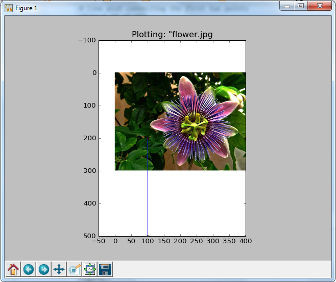
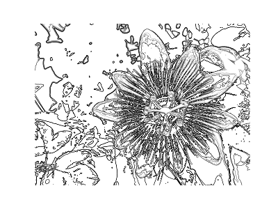
Image Contours
from PIL import Image
from pylab import *
# read image to array
im = array(Image.open('images/flower.jpg').convert('L'))
# create a new figure
figure()
# don’t use colors
gray()
# show contours with origin upper left corner
contour(im, origin='image')
axis('equal')
axis('off')
Histograms:
figure()
hist(im.flatten(),128)
show()
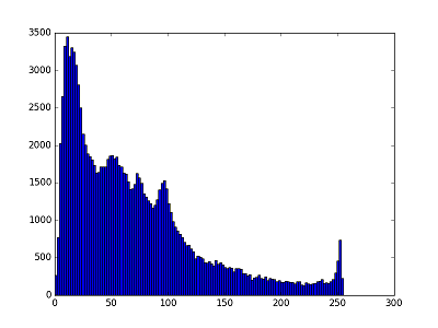 This shows the distribution of pixel values. A number of bins is specified for the span of values and each bin gets a count of how many pixels have values in the bin’s range. The visualization of the (graylevel) image histogram is done using the hist() function.
The second argument specifies the number of bins to use. Note that the image needs to be flattened first, because hist() takes a one-dimensional array as input. The method flatten() converts any array to a one-dimensional array with values taken row-wise.
This shows the distribution of pixel values. A number of bins is specified for the span of values and each bin gets a count of how many pixels have values in the bin’s range. The visualization of the (graylevel) image histogram is done using the hist() function.
The second argument specifies the number of bins to use. Note that the image needs to be flattened first, because hist() takes a one-dimensional array as input. The method flatten() converts any array to a one-dimensional array with values taken row-wise.
Graylevel transforms using NumPy
from PIL import Image
from numpy import *
im = array(Image.open('images/flower.jpg').convert('L'))
im2 = 255 - im #invert image
im3 = (100.0/255) * im + 100 #clamp to interval 100...200
im4 = 255.0 * (im/255.0)**2 #squared
Converting these numpy arrays back into our grayscale images:
npim2 = Image.fromarray(uint8(im2))
npim2.show()
npim3 = Image.fromarray(uint8(im3))
npim3.show()
npim4 = Image.fromarray(uint8(im4))
npim4.show()
Thus the three transformed grayscale images can be compared as follows:

Image De-noising
Image de-noising is the process of removing image noise while at the same time trying to preserve details and structures
from numpy import *

def denoise(im, U_init, tolerance=0.1, tau=0.125, tv_weight=100):
    """ An implementation of the Rudin-Osher-Fatemi (ROF) denoising model
        using the numerical procedure presented in Eq. (11) of A. Chambolle
        (2005). Implemented using periodic boundary conditions
        (essentially turning the rectangular image domain into a torus!).

        Input:
        im - noisy input image (grayscale)
        U_init - initial guess for U
        tv_weight - weight of the TV-regularizing term
        tau - steplength in the Chambolle algorithm
        tolerance - tolerance for determining the stop criterion

        Output:
        U - denoised and detextured image (also the primal variable)
        T - texture residual"""

    #---Initialization
    m,n = im.shape #size of noisy image

    U = U_init
    Px = im #x-component to the dual field
    Py = im #y-component of the dual field
    error = 1
    iteration = 0

    #---Main iteration
    while (error > tolerance):
        Uold = U

        #Gradient of primal variable
        LyU = vstack((U[1:,:],U[0,:])) #Left translation w.r.t. the y-direction
        LxU = hstack((U[:,1:],U.take([0],axis=1))) #Left translation w.r.t. the x-direction

        GradUx = LxU-U #x-component of U's gradient
        GradUy = LyU-U #y-component of U's gradient

        #First we update the dual varible
        PxNew = Px + (tau/tv_weight)*GradUx #Non-normalized update of x-component (dual)
        PyNew = Py + (tau/tv_weight)*GradUy #Non-normalized update of y-component (dual)
        NormNew = maximum(1,sqrt(PxNew**2+PyNew**2))

        Px = PxNew/NormNew #Update of x-component (dual)
        Py = PyNew/NormNew #Update of y-component (dual)

        #Then we update the primal variable
        RxPx =hstack((Px.take([-1],axis=1),Px[:,0:-1])) #Right x-translation of x-component
        RyPy = vstack((Py[-1,:],Py[0:-1,:])) #Right y-translation of y-component
        DivP = (Px-RxPx)+(Py-RyPy) #Divergence of the dual field.
        U = im + tv_weight*DivP #Update of the primal variable

        #Update of error-measure
        error = linalg.norm(U-Uold)/sqrt(n*m);
        iteration += 1;

        print iteration, error

    #The texture residual
    T = im - U
    print 'Number of ROF iterations: ', iteration

    return U,T
In this example, we used the function roll(), which as the name suggests, "rolls" the values of an array cyclically around an axis. This is very convenient for computing neighbor differences, in this case for derivatives. We also used linalg.norm() which measures the difference between two arrays (in this case the image matrices U and Uold)
We can now use the denoise function to remove noise from a real image This is the image to be tested:
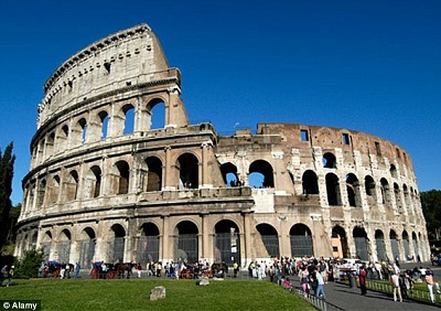
from PIL import Image
import pylab

im = array(Image.open('images/noiseimage.jpg').convert('L'))
U,T = denoise(im,im)

pylab.figure()
pylab.gray()
pylab.imshow(U)
pylab.axis('equal')
pylab.axis('off')
pylab.show()
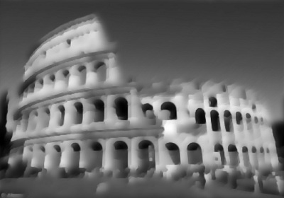
The resulting de-noised image is:
Thus we are done with the basics of Computer Vision. Next we would level up a bit by exploring the OpenCV library.