Digit Recognition using OpenCV and Scikit-Learn
The Problem:
Digit recognition is the ability of a computer to receive and interpret intelligible handwritten numerical input from sources such as paper documents, images, touch-screens and other devices. In this example, we will see how to build a digit recognizer application that takes the input of an image and recognizes the handwritten digits in that image.
The Data Set:
The data used for this problem is the classical MNIST ("Modified National Institute of Standards and Technology") dataset which is extensively studied in the Machine Learning Community.
The MNIST database is a set of 70000 samples of handwritten digits where each sample consists of 28×28 sized grayscale images. We will be using sklearn.datasets package to download the MNIST database.
Step 1. Training the Digit Classifier:
Here, we will : –
- Calculate the Histogram of Oriented Gaussians(HOG) features for each sample in the database.
- Train a multi-class linear SVM with the HOG features of each sample along with the corresponding label.
- Save the classifier in a file so that we can use the classifier again without performing training each time.
# Importing the modules
from sklearn.externals import joblib
from sklearn import datasets
from skimage.feature import hog
from sklearn.svm import LinearSVC
import numpy as np
from collections import Counter

# Load the dataset
# This might take some time as a process of downloading about 55mb of data would be going on.
dataset = datasets.fetch_mldata("MNIST Original")

# Once, the dataset is downloaded we will save the images of the digits in a numpy array features and the corresponding labels
# i.e. the digit in another numpy array labels
# Extract the features and labels
features = np.array(dataset.data, 'int16')
labels = np.array(dataset.target, 'int')

# Calculate the HOG features for each image in the database and save them in another numpy array named hog_feature.
list_hog_fd = []
for feature in features:
    fd = hog(feature.reshape((28, 28)), orientations=9, pixels_per_cell=(14, 14), cells_per_block=(1, 1), visualise=False)
    list_hog_fd.append(fd)
hog_features = np.array(list_hog_fd, 'float64')

print "Count of digits in dataset", Counter(labels)

# The next step is to create a Linear SVM object. Since there are 10 digits, we need a multi-class classifier.
# The Linear SVM that comes with sklearn can perform multi-class classification.
clf = LinearSVC()

# Perform the training using the fit function of clf
clf.fit(hog_features, labels)

# Save the classifier
joblib.dump(clf, "digits_cls.pkl", compress=3)
The crux of this code to tain our digit classifier after the initial loading of digit dataset and extracting the features and labels, is extracting the HOG features.
The arguments passed in the hog() functions are explained below:
We set the number of cells in each block equal to one and each individual cell is of size 14×14. Since our image is of size 28×28, we will have four blocks/cells of size 14×14 each. Also, we set the size of orientation vector equal to 9. So our HOG feature vector for each sample will be of size 4×9 = 36. We are not interesting in visualizing the HOG feature image, so we will set the visualise parameter to false.
After this step we create the LinearSVM() object to do multi-classification.
Then we train our classifier using the fit() function which takes two parameters:
- an array of the HOG features of the handwritten digit earlier calculated
- Corresponding array of labels. Each label value is from the set — [0, 1, 2, 3,…, 8, 9].
When the training finishes, we will save the classifier in a file named digitscls.pkl using _joblib.dump() function which has parameters of:
- The classifier object
- Filename where we want to save the classifier
- The compression degree ranging from 0-9. 0 means no compression whereas higher degree means more compression althoug poor computation time. Results have show compression = 3 proves to be a good trade-off.
Thus we have successfully trained our digits classifier.
Step2. Recognizing digits using our classifier:
Now that our classifeir is ready, we can test it on an input of actual digits.
import cv2
from sklearn.externals import joblib
from skimage.feature import hog
import numpy as np

# Load the classifier
clf = joblib.load("digits_cls.pkl")

# Read the input image
im = cv2.imread("images/hdigits.jpg")

# Convert to grayscale and apply Gaussian filtering
im_gray = cv2.cvtColor(im, cv2.COLOR_BGR2GRAY)
im_gray = cv2.GaussianBlur(im_gray, (5, 5), 0)

# Threshold the image
ret, im_th = cv2.threshold(im_gray, 90, 255, cv2.THRESH_BINARY_INV)

# Find contours in the image
_,ctrs,_ = cv2.findContours(im_th.copy(), cv2.RETR_EXTERNAL, cv2.CHAIN_APPROX_SIMPLE)

# Get rectangles contains each contour
rects = [cv2.boundingRect(ctr) for ctr in ctrs]

# For each rectangular region, calculate HOG features and predict
# the digit using Linear SVM.
for rect in rects:
    # Draw the rectangles
    cv2.rectangle(im, (rect[0], rect[1]), (rect[0] + rect[2], rect[1] + rect[3]), (0, 255, 0), 3)
    # Make the rectangular region around the digit
    leng = int(rect[3] * 1.6)
    pt1 = int(rect[1] + rect[3] // 2 - leng // 2)
    pt2 = int(rect[0] + rect[2] // 2 - leng // 2)
    roi = im_th[pt1:pt1+leng, pt2:pt2+leng]
    # Resize the image
    roi = cv2.resize(roi, (28, 28), interpolation=cv2.INTER_AREA)
    roi = cv2.dilate(roi, (3, 3))
    # Calculate the HOG features
    roi_hog_fd = hog(roi, orientations=9, pixels_per_cell=(14, 14), cells_per_block=(1, 1), visualise=False)
    nbr = clf.predict(np.array([roi_hog_fd], 'float64'))
    cv2.putText(im, str(int(nbr[0])), (rect[0], rect[1]),cv2.FONT_HERSHEY_DUPLEX, 2, (0, 255, 255), 3)

cv2.imshow("Digit Recognizer", im)
cv2.waitKey()
For testing our calssifier on real input, we loaded the classifier from the file digits_cls.pkl which we had saved in the previous script.
Then we load the test image, convert it to a grayscale image as we have seen before and then apply a Gaussian filter to it so for smoothing.
Next we convert our grayscale image into a binary image using a threshold value of 90. All the pixel locations with grayscale values greater than 90 are set to 0(black)in the binary image and all the pixel locations with grayscale values less than 90 are set to 255(white) in the binary image.
We calculate the contours in the image, calculate the bounding box for each contour and then generate a bounding square around each contour for each corresponding bounding box.
Next we then resize each bounding square to a size of 28×28 and dilate it.
We calculate the HOG features for each bounding square. (The HOG feature vector for each bounding square should be of the same size for which the classifier was trained, else you will get an error).
Finally, we predict the digit using our classifier. We also draw the bounding box and the predicted digit on the input image. and then display the image.
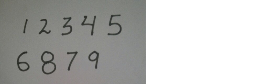
I tested the classifier on this image -
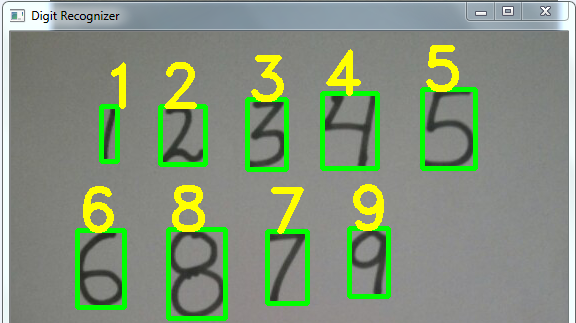
The resulting output with the digits recognized looked like this:
NOTE: While using your own images for testing:
Make sure each is at a sufficient distance from each other. Otherwise if the digits are too close, they will interfere in the square region around each digit. In this case, we will need to create a new square image and then we need to copy the contour in that square image.
For the images I used in testing, fixed thresholding worked pretty well. In most real world images, fixed thresholding does not produce good results. In this case, we need to use adaptive thresholding.
In the pre-processing step, we only did Gaussian blurring. In most situations, on the binary image we will need to open and close the image to remove small noise pixels and fill small holes ie perform appropriate Image Denoising and Inpainting.
Thus here we discussed how we can recognize handwritten digits using OpenCV and Scikit-Learn. We trained a Linear SVM with the HOG features of each sample and then ultimately tested our code.