Feature Detection and Description¶

In computer vision and image processing the concept of feature detection refers to methods that aim at computing abstractions of image information and making local decisions at every image point whether there is an image feature of a given type at that point or not. The resulting features will be subsets of the image domain, often in the form of isolated points, continuous curves or connected regions. Feature detection can include detecting edges, some defined patches in the images, center or the corners of the image. Of these while Image Processing, the patches are flat and are difficut to track. As we move verticalling while processing then edges would change, from bottom edge to a left (or right upward edge). Hence these would be difficult to extract. Whereas while processing corners each patch of the corner to be processed would be different from eaach other and hence it would be easier to track. Blobs are another type of features which prove effective for extraction.

For finding these features, we look for the regions in images which have maximum variation when moved (by a small amount) in all regions around it. Finding these image features is called Feature Detection. Description of the region around the feature by the computer, so that it could find it in other images is called Feature Description.

Below we will take a look at few of the techniques used for Feature Detection and Description mainly Corner Detections and Feature Matching.

Corner Detection¶

1] Harris Corner Detector in OpenCV:¶

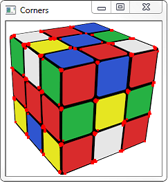
OpenCV has the function cv2.cornerHarris() for this purpose. Its arguments are :

img - Input image, it should be grayscale and float32 type.
blockSize - It is the size of neighbourhood considered for corner detection
ksize - Aperture parameter of Sobel derivative used.
k - Harris detector free parameter in the equation.

import cv2
import numpy as np
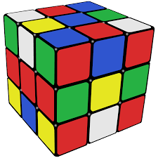
filename = 'images/cube.png'
img = cv2.imread(filename)
gray = cv2.cvtColor(img,cv2.COLOR_BGR2GRAY)
gray = np.float32(gray)
dst = cv2.cornerHarris(gray,2,3,0.04)

#result is dilated for marking the corners, not important
dst = cv2.dilate(dst,None)

# Threshold for an optimal value, it may vary depending on the image.
img[dst>0.01*dst.max()]=[0,0,255]
cv2.imshow('Corners',img)

if cv2.waitKey(0) & 0xff == 27:
    cv2.destroyAllWindows()

I used an image of a cube. Feel free to test any image you like:

Corner with SubPixel Accuracy¶

Sometimes, you may need to find the corners with maximum accuracy. OpenCV comes with a function cv2.cornerSubPix() which further refines the corners detected with sub-pixel accuracy.First we find the corners using the above Harris Corner Detector. Then we pass the centroids of these corners to refine them. Harris corners are marked in red pixels and refined corners are marked in green pixels. For this function, we have to define the criteria when to stop the iteration. We stop it after a specified number of iteration or a certain accuracy is achieved, whichever occurs first. We also need to define the size of neighbourhood it would search for corners.

import cv2
import numpy as np
filename = 'images/cube.png'
img = cv2.imread(filename)
gray = cv2.cvtColor(img,cv2.COLOR_BGR2GRAY)

# find Harris corners
gray = np.float32(gray)
dst = cv2.cornerHarris(gray,2,3,0.04)
dst = cv2.dilate(dst,None)
ret, dst = cv2.threshold(dst,0.01*dst.max(),255,0)
dst = np.uint8(dst)

# find centroids
ret, labels, stats, centroids = cv2.connectedComponentsWithStats(dst)

# define the criteria to stop and refine the corners
criteria = (cv2.TERM_CRITERIA_EPS + cv2.TERM_CRITERIA_MAX_ITER, 100, 0.001)
corners = cv2.cornerSubPix(gray,np.float32(centroids),(5,5),(-1,-1),criteria)

# Now draw them
res = np.hstack((centroids,corners))
res = np.int0(res)
img[res[:,1],res[:,0]]=[0,0,255]
img[res[:,3],res[:,2]] = [0,0,255]

cv2.imshow('Corners',img)

The resulting image would look like:

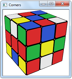
As you can see the corners are crisp and sharp.

2] Shi-Tomasi Corner Detector & Good Features to Track¶

OpenCV has a function, cv2.goodFeaturesToTrack(). It finds N strongest corners in the image by Shi-Tomasi method (or Harris Corner Detection, if you specify it). As usual, image should be a grayscale image. Then you specify number of corners you want to find. Then you specify the quality level, which is a value between 0-1, which denotes the minimum quality of corner below which everyone is rejected. Then we provide the minimum euclidean distance between corners detected.

With all these informations, the function finds corners in the image. All corners below quality level are rejected. Then it sorts the remaining corners based on quality in the descending order. Then function takes first strongest corner, throws away all the nearby corners in the range of minimum distance and returns N strongest corners.

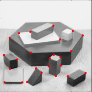
In below example, we will try to find 25 best corners:

import numpy as np
import cv2
from matplotlib import pyplot as plt

img = cv2.imread('images/shapes.jpg')
gray = cv2.cvtColor(img,cv2.COLOR_BGR2GRAY)

corners = cv2.goodFeaturesToTrack(gray,25,0.01,10)
corners = np.int0(corners)

for i in corners:
    x,y = i.ravel()
    cv2.circle(img,(x,y),3,255,-1)    

plt.imshow(img),plt.show()

The resulting image would look like:

SIFT (Scale-Invariant Feature Transform)¶

In last couple of chapters, we saw some corner detectors like Harris, Shi Tomasi etc. They are rotation-invariant, which means, even if the image is rotated, we can find the same corners. It is obvious because corners remain corners in rotated image also. But what about scaling? A corner may not be a corner if the image is scaled. A corner in a small image within a small window is flat when it is zoomed in the same window. So Harris corner is not scale invariant.

There are mainly four steps involved in SIFT algorithm:

Scale-space Extrema Detection: Due to scale-variance we can't use the same window to detect keypoints with different scale. It is OK with small corner. But to detect larger corners we need larger windows. For this, scale-space filtering is used.
Keypoint Localization: Once potential keypoints locations are found, they have to be refined to get more accurate results. They used Taylor series expansion of scale space to get more accurate location of extrema, and if the intensity at this extrema is less than a threshold value (0.03 generally), it is rejected. This threshold is called contrastThreshold in OpenCV.
Orientation Assignment: Now an orientation is assigned to each keypoint to achieve invariance to image rotation. A neigbourhood is taken around the keypoint location depending on the scale, and the gradient magnitude and direction is calculated in that region
Keypoint Descriptor Now keypoint descriptor is created. A 16x16 neighbourhood around the keypoint is taken. It is devided into 16 sub-blocks of 4x4 size. For each sub-block, 8 bin orientation histogram is created. So a total of 128 bin values are available. It is represented as a vector to form keypoint descriptor. In addition to this, several measures are taken to achieve robustness against illumination changes, rotation etc.
Keypoint Matching Keypoints between two images are matched by identifying their nearest neighbours. But in some cases, the second closest-match may be very near to the first. It may happen due to noise or some other reasons. In that case, ratio of closest-distance to second-closest distance is taken. If it is greater than 0.8, they are rejected. It eliminaters around 90% of false matches while discards only 5% correct matches.

This is a summary of SIFT algorithm. For more details and understanding, reading the original paper is highly recommended. Now we'll see how SIFT can be implemented using OpenCV:

import cv2
import numpy as np
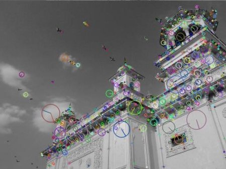
img = cv2.imread('images/building.jpg')
gray= cv2.cvtColor(img,cv2.COLOR_BGR2GRAY)
sift = cv2.SIFT()
kp = sift.detect(gray,None)
img=cv2.drawKeypoints(gray,kp)
cv2.imwrite('sift_keypoints.jpg',img)

sift.detect() function finds the keypoint in the images. You can pass a mask if you want to search only a part of image. Each keypoint is a special structure which has many attributes like its (x,y) coordinates, size of the meaningful neighbourhood, angle which specifies its orientation, response that specifies strength of keypoints etc.

OpenCV also provides cv2.drawKeyPoints() function which draws the small circles on the locations of keypoints. If you pass a flag, cv2.DRAW_MATCHES_FLAGS_DRAW_RICH_KEYPOINTS to it, it will draw a circle with size of keypoint and it will even show its orientation. See below example.

img=cv2.drawKeypoints(gray,kp,flags=cv2.DRAW_MATCHES_FLAGS_DRAW_RICH_KEYPOINTS)
cv2.imwrite('sift_keypoints.jpg',img)

The resulting image would look like:

Now to calculate the descriptor, OpenCV provides two methods.

Since you already found keypoints, you can call sift.compute() which computes the descriptors from the keypoints we have found. Eg: kp,des = sift.compute(gray,kp)
If you didn't find keypoints, directly find keypoints and descriptors in a single step with the function, sift.detectAndCompute(). The second method is shown below:

sift = cv2.SIFT()
kp, des = sift.detectAndCompute(gray,None)

SURF (Speeded-Up Robust Features)¶

Implementing SIFT for Feature Detection and Description is quite slow and hence an update was required. The SURF (Speeded-Up Robust Features) provides this update. SURF adds a lot of features to improve the speed in every step. Analysis shows it is 3 times faster than SIFT while performance is comparable to SIFT. SURF is good at handling images with blurring and rotation, but not good at handling viewpoint change and illumination change. Below code shows implementation of SURF using OpenCV

img = cv2.imread('fly.png',0)

# Create SURF object. You can specify params here or later.
# Here I set Hessian Threshold to 400
surf = cv2.SURF(400)

# Find keypoints and descriptors directly
kp, des = surf.detectAndCompute(img,None)

len(kp)

699

This much keypoints is too much to show in a picture. We reduce it to some 50 to draw it on an image. While matching, we may need all those features, but not now. So we increase the Hessian Threshold.

# Check present Hessian threshold
print surf.hessianThreshold

400

# We set it to some 50000. Remember, it is just for representing in picture.
# In actual cases, it is better to have a value 300-500
surf.hessianThreshold = 50000

# Again compute keypoints and check its number.
kp, des = surf.detectAndCompute(img,None)
print len(kp)

47

It is less than 50. Now we can draw it on the image:

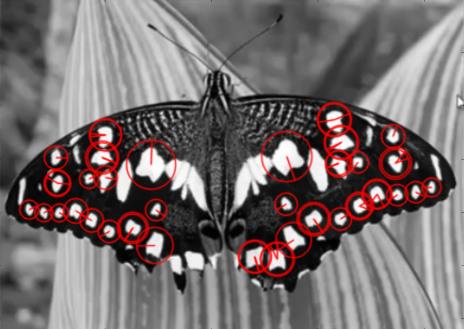
img2 = cv2.drawKeypoints(img,kp,None,(255,0,0),4)
plt.imshow(img2),plt.show()

Observing the below resulting image, we can infer SURF is more like a blob detector. It detects the white blobs on wings of butterfly. Feel free to test it with other images too.

If you want to apply U-SURF, so that it won't find the orientation:

# Check upright flag, if it False, set it to True
print surf.upright

False

surf.upright = True

# Recompute the feature points and draw it
kp = surf.detect(img,None)
img2 = cv2.drawKeypoints(img,kp,None,(255,0,0),4)
plt.imshow(img2),plt.show()

See the results below. All the orientations are shown in same direction. It is more faster than previous. If you are working on cases where orientation is not a problem (like panorama stitching) etc, this is better.

Finally we check the descriptor size and change it to 128 if it is only 64-dim.

# Find size of descriptor
print surf.descriptorSize()

64

# That means flag, "extended" is False.
surf.extended

False

# So we make it to True to get 128-dim descriptors.
surf.extended = True
kp, des = surf.detectAndCompute(img,None)
print surf.descriptorSize()

128

print des.shape

(47,128)

FAST Algorithm for Corner Detection¶

We saw several feature detectors and many of them are really good. But when looking from a real-time application point of view, they are not fast enough. One best example would be SLAM (Simultaneous Localization and Mapping) mobile robot which have limited computational resources.

As a solution to this, FAST (Features from Accelerated Segment Test) algorithm was proposed by Edward Rosten and Tom Drummond in their paper "Machine learning for high-speed corner detection" in 2006 (Later revised it in 2010). Refer original paper for more details (All the images are taken from original paper).

This algorithm proved to be several times faster than other existing corner detectors. However it is not robust to high levels of noise. It is dependant on a threshold.

It is called as any other feature detector in OpenCV. If you want, you can specify the threshold, whether non-maximum suppression to be applied or not, the neighborhood to be used etc.

For the neighborhood, three flags are defined, cv2.FAST_FEATURE_DETECTOR_TYPE_5_8, cv2.FAST_FEATURE_DETECTOR_TYPE_7_12 and cv2.FAST_FEATURE_DETECTOR_TYPE_9_16. Below is a simple code on how to detect and draw the FAST feature points.

import numpy as np
import cv2
from matplotlib import pyplot as plt

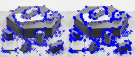
img = cv2.imread('simple.jpg',0)

# Initiate FAST object with default values
fast = cv2.FastFeatureDetector()

# find and draw the keypoints
kp = fast.detect(img,None)
img2 = cv2.drawKeypoints(img, kp, color=(255,0,0))

# Print all default params
print "Threshold: ", fast.getInt('threshold')
print "nonmaxSuppression: ", fast.getBool('nonmaxSuppression')
print "neighborhood: ", fast.getInt('type')
print "Total Keypoints with nonmaxSuppression: ", len(kp)

cv2.imwrite('fast_true.png',img2)

# Disable nonmaxSuppression
fast.setBool('nonmaxSuppression',0)
kp = fast.detect(img,None)

print "Total Keypoints without nonmaxSuppression: ", len(kp)

img3 = cv2.drawKeypoints(img, kp, color=(255,0,0))

cv2.imwrite('fast_false.png',img3)

The resulting image would look like the following. First image shows FAST with nonmaxSuppression and second one without nonmaxSuppression:

Feature Matching¶

Here we will see Feature matching, which is in one way or the other similiar to template matching but as you will see gives impressive and better results than the latter.

The process is the same, we take a template image, one that we want to find, and then we can search for this image in some another image. The difference between Feature Matching and Template Matching is that the images not need to be the same lighting, angle, rotation...etc. Just the features need to match up. Now to match these features we would be using a Brute-Force Matcher.

Here is the template image of a notebook I would be using to test the Brute-Force Matcher.

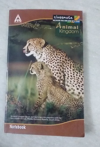
And the two images to be searched are:

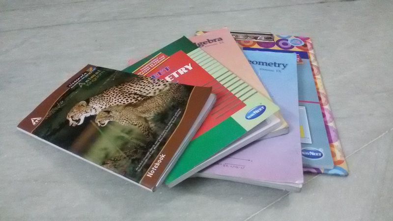
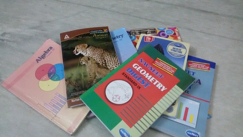
I basically rearranged the notebooks to extensively test the code. As you will see neither the lighting conditions nor the position of the images matter while matching.

Let's get started with the code. Initially as always, importing our modules and our test images:

import numpy as np
import cv2
import matplotlib.pyplot as plt

img1 = cv2.imread('template.jpg',0)
#img2 = cv2.imread('image1.jpg',0)
img2 = cv2.imread('image2.jpg',0)

We will use the ORB (Oriented FAST and Rotated BRIEF) detector to find the key points and their descriptions. ORB which is a fast robust local feature detector. It has a similiar function as SIFT and SURF but unlike them, it isn't patented and is free to use.

orb = cv2.ORB_create()

kp1, des1 = orb.detectAndCompute(img1,None)
kp2, des2 = orb.detectAndCompute(img2,None)

Now we match the features using the Brute Force Matcher. Brute-Force matcher takes the descriptor of one feature in first set and is matched with all other features in second set using some distance calculation. And the closest one is returned.

For BF matcher, first we have to create the BFMatcher object using cv2.BFMatcher(). It takes two optional params.

normType. It specifies the distance measurement to be used. By default, it is cv2.NORM_L2. It is good for SIFT, SURF etc (cv2.NORM_L1 is also there). For binary string based descriptors like ORB, BRIEF, BRISK etc, cv2.NORM_HAMMING should be used, which used Hamming distance as measurement. If ORB is using VTA_K == 3 or 4, cv2.NORM_HAMMING2 should be used.
crossCheck It is a boolean variable - false by default. If it is true, Matcher returns only those matches with value (i,j) such that i-th descriptor in set A has j-th descriptor in set B as the best match and vice-versa. That is, the two features in both sets should match each other. It provides consistant result, and is a good alternative to ratio test proposed by D.Lowe in SIFT paper.

Once it is created, two important methods are BFMatcher.match() and BFMatcher.knnMatch(). First one returns the best match. Second method returns k best matches where k is specified by the user. It may be useful when we need to do additional work on that.

We use the function cv2.drawMatches() to draw the matches. It stacks two images horizontally and draw lines from first image to second image showing best matches. We can and should limit the matches to be drawn to something around 10 or 20, The more number of matches specified, the more will be the computation time. Thus 20 matches seems to be a fair bet.

bf = cv2.BFMatcher(cv2.NORM_HAMMING, crossCheck=True) 

# Here we create matches of the descriptors and then we sort them based on their distances.
matches = bf.match(des1,des2)
matches = sorted(matches, key = lambda x:x.distance)

# Then finally draw the first 20 matches and show the resulting images.
img3 = cv2.drawMatches(img1,kp1,img2,kp2,matches[:20],None, flags=2)
plt.imshow(img3)
plt.show()

The resulting outputs with the features matched are:

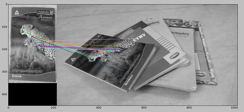
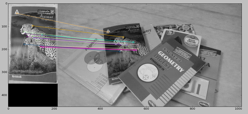
As you can see, barring a few feature points, most of the features were correctly matched and the template notebook image was effectively found in both the images irrespective of the different shadows, lightning, rotation and positions. Similiar techniques can be implemented for making a small scale image browser or a book-cover matcher for Amazon where you input an image of a cover of a book you want and then, search results of the actual book would be returned. Possibilities are unlimited.