Video Analysis
Here we would be dealing with analysis of videos and it's various aspects like object tracking, optical flow and background reduction. OpenCV can be effectively used for analysis of real-time as well as non real-time (I don't know if it's a word, but I think you get the idea..) videos. Hence we would see different functions and algorithms defined in OpenCV related to Video Processing in the following:
Object Tracking in videos
To track objects and their movements in video feeds, we would be using and comparing two different techniques defined in OpenCV.
- Mean Shift Tracking
- Camshift Tracking
Mean Shift Tracking
Suppose you have a set of points (it can be a pixel distribution like histogram backprojection) and you are given a small window (like a rectangle). Now you want to move that window to the area of maximum pixel density (or maximum number of points). This is where Meanshift Tracking would be used.
In Meanshift Tracking we normally pass the histogram backprojected image and initial target location. When the object moves, obviously the movement is reflected in histogram backprojected image. As a result, meanshift algorithm moves our window to the new location with maximum density.
To use meanshift in OpenCV, first we need to setup the target, find its histogram so that we can backproject the target on each frame for calculation of meanshift. We also need to provide initial location of window. For histogram, only Hue is considered here. Also, to avoid false values due to low light, low light values are discarded using cv2.inRange() function.
The following code shows an example where Meanshift Tracking is used to track cars in a video of expressway traffic. The video to be used as the input is:
from IPython.display import HTML
HTML("""
<video controls>
  <source src="videos/slow_traffic.mp4" type="video/mp4">
</video>
""")
# import numpy as np
import cv2
cap = cv2.VideoCapture('slow_traffic.mp4')

# take first frame of the video
ret,frame = cap.read()

# setup initial location of window
r,h,c,w = 200,20,300,20  # simply hardcoded the values
track_window = (c,r,w,h)

# set up the ROI for tracking
roi = frame[r:r+h, c:c+w]
hsv_roi = cv2.cvtColor(frame, cv2.COLOR_BGR2HSV)
mask = cv2.inRange(hsv_roi, np.array((0., 60.,32.)), np.array((180.,255.,255.)))
roi_hist = cv2.calcHist([hsv_roi],[0],mask,[180],[0,180])
cv2.normalize(roi_hist,roi_hist,0,255,cv2.NORM_MINMAX)
The function calcHist() used here calculates the histogram of one or more arrays. The elements of a tuple used to increment a histogram bin are taken from the corresponding input arrays at the same location. It's parameters are:
- images - Source arrays. They all should have the same depth, CV_8U or CV_32F, and the same size. Each of them can have an arbitrary number of channels.
- nimages - Number of source images.
- channels - List of the dims channels used to compute the histogram. The first array channels are numerated from 0 to images[0].channels()-1 , the second array channels are counted from images[0].channels() to images[0].channels() + images[1].channels()-1, and so on.
- mask - Optional mask. If the matrix is not empty, it must be an 8-bit array of the same size as images[i] . The non-zero mask elements mark the array elements counted in the histogram.
- hist - Output histogram, which is a dense or sparse dims -dimensional array.
- dims - Histogram dimensionality that must be positive and not greater than CV_MAX_DIMS (equal to 32 in the current OpenCV version).
- histSize - Array of histogram sizes in each dimension.
- ranges - Array of the dims arrays of the histogram bin boundaries in each dimension.
# Setup the termination criteria, either 10 iteration or move by atleast 1 pt
term_crit = ( cv2.TERM_CRITERIA_EPS | cv2.TERM_CRITERIA_COUNT, 10, 1 )
while(1):
    ret ,frame = cap.read()

    if ret == True:
        hsv = cv2.cvtColor(frame, cv2.COLOR_BGR2HSV)
        dst = cv2.calcBackProject([hsv],[0],roi_hist,[0,180],1)

        # apply meanshift to get the new location
        ret, track_window = cv2.meanShift(dst, track_window, term_crit)

        # Draw it on image
        x,y,w,h = track_window
        img2 = cv2.rectangle(frame, (x,y), (x+w,y+h), 255,2)
        cv2.imshow('img2',img2)

        k = cv2.waitKey(60) & 0xff
        if k == 27:
            break
        else:
            cv2.imwrite(chr(k)+".jpg",img2)

    else:
        break

cv2.destroyAllWindows()
cap.release()
The functions calcBackProject() calculates the back project of the histogram. Similar to calcHist(), at each location (x, y), the function collects the values from the selected channels in the input images and finds the corresponding histogram bin. However instead of incrementing it, the function reads the bin value, scales it by scale, and stores in backProject(x,y).
Then we use the meanshift() function. It's parameters are:
- probImage - Back projection of the object histogram.
- window - Initial search window.
- criteria - Stop criteria for the iterative search algorithm.
The resulting output of the code is:
HTML("""
<video controls>
  <source src="videos/meanshiftoutput.mp4" type="video/mp4">
</video>
""")
There is one problem with Mean Shift. Our window always has the same size when car is farther away and it is very close to camera. That is not good. We need to adapt the window size with size and rotation of the target. To overcome this problem OpenCV has another technique called CAMshift (Continuous Adaptive Mean Shift).
CamShift Tracking
The CamShift algorithm is iterative, meaning that it seeks to optimize the tracking criterion. In this case, we’ll set the termination criterion to perform two checks.
- The first check is the epsilon associated with the centroids of our selected ROI and the tracked ROI according to the CamShift algorithm. If the tracked centroid has not changed by at least one pixel, then terminate the CamShift algorithm.
- The second check controls the number of iterations of CamShift. Using more iterations will allow CamShift to (ideally) find a closer centroid match between the selected ROI and the tracked ROI; however, this comes at the cost of runtime. If the iterations are set too high, then we will drop below real-time performance, which is substantially less than ideal in most situations. Let’s go ahead and use a maximum of 10 iterations so we don’t fall into this scenario.
CAMShift expects three arguments:
- backProj: Which is the output of the histogram back projection.
- roiBox: The estimated bounding box containing the object that we want to track.
- termination: Our termination criterion which we defined
The steps followed in applying CAMShift are as follows:
- Capture the frames form the camera. Get the initial ROI of the region to be tracked. For each frame -
- Get the HSV histogram for the ROI.
- Normalize the histogram.
- Convert the frame into the HSV color space.
- Calculate the backprojection of the histogram of the ROI to be tracked on the HSV frame.
- Apply the CAMshift on the resulting backprojected image with the initial ROI location to get a new location to use in the feedback loop.
Following code shows the implementation of this algorithm:
import numpy as np
import cv2
cap = cv2.VideoCapture('videos/slow_traffic.mp4')

# take first frame of the video
ret,frame = cap.read()

# setup initial location of window
r,h,c,w = 250,40,400,80 # simply hardcoded the values
track_window = (c,r,w,h)

# set up the ROI for tracking
roi = frame[r:r+h, c:c+w]
hsv_roi = cv2.cvtColor(frame, cv2.COLOR_BGR2HSV)
mask = cv2.inRange(hsv_roi, np.array((0., 60.,32.)), np.array((180.,255.,255.)))
roi_hist = cv2.calcHist([hsv_roi],[0],mask,[180],[0,180])
cv2.normalize(roi_hist,roi_hist,0,255,cv2.NORM_MINMAX)

# Setup the termination criteria, either 10 iteration or move by atleast 1 pt
term_crit = ( cv2.TERM_CRITERIA_EPS | cv2.TERM_CRITERIA_COUNT, 10, 1 )

while(1):
    ret ,frame = cap.read()

    if ret == True:
        hsv = cv2.cvtColor(frame, cv2.COLOR_BGR2HSV)
        dst = cv2.calcBackProject([hsv],[0],roi_hist,[0,180],1)

        # apply meanshift to get the new location
        ret, track_window = cv2.CamShift(dst, track_window, term_crit)

        # Draw it on image
        pts = cv2.boxPoints(ret)
        pts = np.int0(pts)
        img2 = cv2.polylines(frame,[pts],True, 255,2)
        cv2.imshow('img2',img2)
        k = cv2.waitKey(60) & 0xff
        if k == 27:
            break
        else:
            cv2.imwrite(chr(k)+".jpg",img2)

    else:
        break
cv2.destroyAllWindows()
cap.release()
The resulting output video would have the following frames:
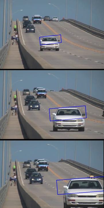
This method involves hardcoding our rectangle which decides the object to be tracked. Sometimes in different conditions, this may become a tedious job, which you might have encountered if you are using your own video as input. A lot of trial and error values have to be used. So instead of that, the following code might prove useful.
It is already documented and self explanatory- pretty much similiar to what we did above. The basic difference is: instead of drawing our own rectangle, we have used a method to stop the video whenever 'i' key is pressed. After that you just have to click at 4 different points on the video to mark your region of interest; this rectangle would then guide the tracking. After drawing those 4 points just click anywhere other than 'i' and the video would continue and the object would be tracked using camshift using the above explained steps. Feel free to use your own videos to test. Also make sure to make the video to run slowly, because this method isn't best suited to track fast moving objects. You can slow down your video using:
cv2.imshow("frame", frame)
cv2.waitKey(25)
# here 25 is the time in milliseconds for which the particular frame would be displayed.
# You can slow down the video by increasing this number accordingly.
Run the following code by specifying the path to the video you want to analyse in camera = cv2.VideoCapture('your/video.mp4'). Once your video is loaded, press the 'i' key and select four points surround the object that you want to track. After your four points are selected, press any key to exit input mode. Now that our script knows what to track and the reference histogram is computed, you should see the object being tracked across the screen in subsequent frames:
import numpy as np
import cv2

# initialize the current frame of the video, along with the list of
# ROI points along with whether or not this is input mode

frame = None  # current frame of the video that we are processing.
roiPts = []  # points corresponding to the Region of Interest (ROI) in our video.
inputMode = False  # indicates whether or not we are currently selecting the object we want to track in the video.

def selectROI(event, x, y, flags, param):
    # grab the reference to the current frame, list of ROI points and whether or not it is ROI selection mode
    global frame, roiPts, inputMode

    # if we are in ROI selection mode, the mouse was clicked,
    # and we do not already have four points, then update the list of ROI points with the (x, y) location of the click
    # and draw the circle
    if inputMode and event == cv2.EVENT_LBUTTONDOWN and len(roiPts) < 4:
        roiPts.append((x, y))
        cv2.circle(frame, (x, y), 4, (0, 255, 0), 2)
        cv2.imshow("frame", frame)

def main():
    # grab the reference to the current frame, list of ROI points and whether or not it is ROI selection mode
    global frame, roiPts, inputMode

    # Supplying our input video
    # If you want you can use VideoCapture(0) to use the webcam
    camera = cv2.VideoCapture('videos/slow_traffic.mp4')

    # setup the mouse callback
    cv2.namedWindow("frame")
    cv2.setMouseCallback("frame", selectROI)

    # initialize the termination criteria for cam shift,
    # indicating a maximum of ten iterations or movement by a least one pixel along with the bounding box of the ROI
    termination = (cv2.TERM_CRITERIA_EPS | cv2.TERM_CRITERIA_COUNT, 10, 1)
    roiBox = None

    # keep looping over the frames
    while True:
        # grab the current frame
        (grabbed, frame) = camera.read()

        # check to see if we have reached the end of the
        # video
        if not grabbed:
            break

        # if the see if the ROI has been computed
        if roiBox is not None:
            # convert the current frame to the HSV color space and perform mean shift
            hsv = cv2.cvtColor(frame, cv2.COLOR_BGR2HSV)
            backProj = cv2.calcBackProject([hsv], [0], roiHist, [0, 180], 1)

            # apply cam shift to the back projection, convert the points to a bounding box, and then draw them
            (r, roiBox) = cv2.CamShift(backProj, roiBox, termination)
            pts = np.int0(cv2.boxPoints(r))
            cv2.polylines(frame, [pts], True, (0, 255, 0), 2)

        # show the frame and record if the user presses a key
        cv2.imshow("frame", frame)
        key = cv2.waitKey(80) & 0xFF

        # handle if the 'i' key is pressed, then go into ROI selection mode
        if key == ord("i") and len(roiPts) < 4:
                        # indicate that we are in input mode and clone the frame
            inputMode = True
            orig = frame.copy()

            # keep looping until 4 reference ROI points have been selected;
            # press any key to exit ROI selction mode once 4 points have been selected
            while len(roiPts) < 4:
                cv2.imshow("frame", frame)
                cv2.waitKey(60)

            # determine the top-left and bottom-right points
            roiPts = np.array(roiPts)
            s = roiPts.sum(axis = 1)
            tl = roiPts[np.argmin(s)]
            br = roiPts[np.argmax(s)]

            # grab the ROI for the bounding box and convert it to the HSV color space
            roi = orig[tl[1]:br[1], tl[0]:br[0]]
            roi = cv2.cvtColor(roi, cv2.COLOR_BGR2HSV)
            #roi = cv2.cvtColor(roi, cv2.COLOR_BGR2LAB)

            # compute a HSV histogram for the ROI and store the bounding box
            roiHist = cv2.calcHist([roi], [0], None, [16], [0, 180])
            roiHist = cv2.normalize(roiHist, roiHist, 0, 255, cv2.NORM_MINMAX)
            roiBox = (tl[0], tl[1], br[0], br[1])

        # if the 'q' key is pressed, stop the loop
        elif key == ord("q"):
            break

    camera.release()
    cv2.destroyAllWindows()

if __name__ == "__main__":
    main()
Optical Flow
Optical flow is the pattern of apparent motion of image objects between two consecutive frames caused by the movemement of object or camera. It is 2D vector field where each vector is a displacement vector showing the movement of points from first frame to second.
Optical flow has many applications in areas like :
- Structure from Motion
- Video Compression
- Video Stabilization ...
The Lucas-Kanade method is one of the methods used to solve the problem of finding optical flow in video frames. The gist of the method is that we give some points to track, we receive the optical flow vectors of those points. For large motion videos we have to use pyramids. As we go up in the pyramid, small motions are removed and large motions becomes small motions. So applying Lucas-Kanade there, we get optical flow along with the scale.
In OpenCV cv2.calcOpticalFlowPyrLK() is used for this purpose. The following code is used to tracks some points in a video. To decide the points, we use cv2.goodFeaturesToTrack(). We take the first frame, detect some Shi-Tomasi corner points in it, then we iteratively track those points using Lucas-Kanade optical flow. For the function cv2.calcOpticalFlowPyrLK() we pass the previous frame, previous points and next frame. It returns next points along with some status numbers which has a value of 1 if next point is found, else zero. We iteratively pass these next points as previous points in next step.
import numpy as np
import cv2
cap = cv2.VideoCapture('videos/slow_traffic.mp4')

# params for ShiTomasi corner detection
feature_params = dict( maxCorners = 100,
                        qualityLevel = 0.3,
                        minDistance = 7,
                        blockSize = 7 )

# Parameters for lucas kanade optical flow
lk_params = dict( winSize = (15,15),
                    maxLevel = 2,
                    criteria = (cv2.TERM_CRITERIA_EPS | cv2.TERM_CRITERIA_COUNT, 10, 0.03))

# Create some random colors
color = np.random.randint(0,255,(100,3))

# Take first frame and find corners in it
ret, old_frame = cap.read()
old_gray = cv2.cvtColor(old_frame, cv2.COLOR_BGR2GRAY)
p0 = cv2.goodFeaturesToTrack(old_gray, mask = None, **feature_params)

# Create a mask image for drawing purposes
mask = np.zeros_like(old_frame)

while(1):
    ret,frame = cap.read()
    frame_gray = cv2.cvtColor(frame, cv2.COLOR_BGR2GRAY)

    # calculate optical flow
    p1, st, err = cv2.calcOpticalFlowPyrLK(old_gray, frame_gray, p0, None, **lk_params)

    # Select good points
    good_new = p1[st==1]
    good_old = p0[st==1]

    # draw the tracks
    for i,(new,old) in enumerate(zip(good_new,good_old)):
        a,b = new.ravel()
        c,d = old.ravel()
        mask = cv2.line(mask, (a,b),(c,d), color[i].tolist(), 2)
        frame = cv2.circle(frame,(a,b),5,color[i].tolist(),-1)
    img = cv2.add(frame,mask)

    cv2.imshow('frame',img)
    k = cv2.waitKey(30) & 0xff
    if k == 27:
        break

    # Now update the previous frame and previous points
    old_gray = frame_gray.copy()
    p0 = good_new.reshape(-1,1,2)

cv2.destroyAllWindows()
cap.release()
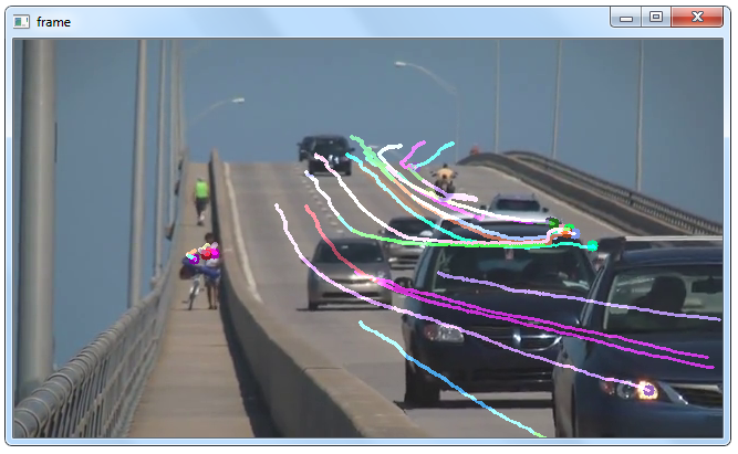
A frame from the resulting output video would show the optical flow as follows:
Dense Optical Flow in OpenCV
Lucas-Kanade method computes optical flow for a sparse feature set (in our example, corners detected using Shi-Tomasi algorithm). OpenCV provides another algorithm to find the dense optical flow. It computes the optical flow for all the points in the frame.
The following code shows how to find dense optical flow. We get a 2-channel array with optical flow vectors, (u,v). We find their magnitude and direction. We color code the result for better visualization. Direction corresponds to Hue value of the image. Magnitude corresponds to Value plane.
Here I used the slow-motion video of landing of a sparrow from youtube.com/user/ultraslo. I say it everytime, feel free to use your own videos. This time too, I won't be any different, except this time, make sure you download the following video and have a look at the amazing result yourself! :P This is the video I downloaded and used:
HTML("""
<video controls>
  <source src="videos/sparrow.mp4" type="video/mp4">
</video>
""")
import cv2
import numpy as np
cap = cv2.VideoCapture("sparrow.mp4")

ret, frame1 = cap.read()
prvs = cv2.cvtColor(frame1,cv2.COLOR_BGR2GRAY)
hsv = np.zeros_like(frame1)
hsv[...,1] = 255

while(1):
    ret, frame2 = cap.read()
    next = cv2.cvtColor(frame2,cv2.COLOR_BGR2GRAY)

    flow = cv2.calcOpticalFlowFarneback(prvs,next, None, 0.5, 3, 15, 3, 5, 1.2, 0)

    mag, ang = cv2.cartToPolar(flow[...,0], flow[...,1])
    hsv[...,0] = ang*180/np.pi/2
    hsv[...,2] = cv2.normalize(mag,None,0,255,cv2.NORM_MINMAX)
    rgb = cv2.cvtColor(hsv,cv2.COLOR_HSV2BGR)

    cv2.imshow('frame2',rgb)
    k = cv2.waitKey(30) & 0xff
    if k == 27:
        break

    elif k == ord('s'):
        cv2.imwrite('opticalfb.png',frame2)
        cv2.imwrite('opticalhsv.png',rgb)
    prvs = next

cap.release()
cv2.destroyAllWindows()
A frame of the resulting output looked like this:
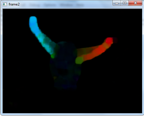
The dense optical flow of the landing sparrow looks totally amazing! :D
Background Subtraction
Background subtraction is a major preprocessing steps in many vision based applications. For example, consider the cases like analyzing human activities from a live feed or that of a visitor counter where a static camera takes the number of visitors entering or leaving the room, or a traffic camera extracting information about the vehicles etc. In all these cases, basically you need to extract the moving foreground from static background.
Cases where we have the image of background alone, like image of the room without visitors, image of the road without vehicles etc, we simply have to subtract the new image from the background. You get the foreground objects alone. However in most of the cases, you may not have such an image, so we need to extract the background from whatever images we have.
BackgroundSubtractorMOG
It is a Gaussian Mixture-based Background/Foreground Segmentation Algorithm. While using this method, we need to create a background object using the function, cv2.createBackgroundSubtractorMOG(). It has optional parameters like length of history, number of gaussian mixtures, threshold etc. which are all set to their default values. Then inside the video loop, use backgroundsubtractor.apply() method to get the foreground mask.
The following example shows the implementation of this algorithm:
import numpy as np
import cv2

#cap = cv2.VideoCapture('slow_traffic.mp4')
cap = cv2.VideoCapture('sparrow.mp4')
fgbg = cv2.createBackgroundSubtractorMOG2()

while(1):
    ret, frame = cap.read()

    fgmask = fgbg.apply(frame)

    cv2.imshow('fgmask',frame)
    cv2.imshow('frame',fgmask)


    k = cv2.waitKey(30) & 0xff
    if k == 27:
        break

cap.release()
cv2.destroyAllWindows()
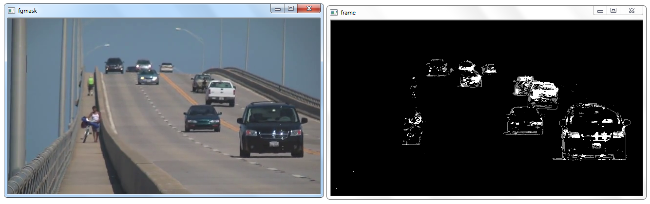
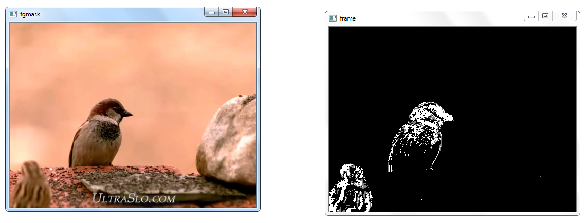
I tested this code on our initial slow_traffic video and the sparrow one. The result was background reduction of each frame in the videos and the comparison between two individual frames looked like the following: